How To Add Drop Down Filter In Excel

This postal service shows how to create multiple dependent drop downs using the FILTER office. These are also known as cascading or conditional drop downs, where the choices in a drop down depend on the selection made in a previous drop down. The technique presented enables you to create as many drop downs as you need, and there is no VBA coding needed.

Note: depending on your version of Excel, you may not have admission to the FILTER, UNIQUE, or SORT functions. If non, check out this post which uses legacy functions or this post which uses slicers.

Objective

Before we get into the mechanics, permit'south clarify our goal. We would like to create a serial of dependent drib downs, where the choices available in a driblet down depend on the option made in a previous drop downwardly.

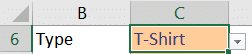
For example, we would similar the user to pick a Type of shirt. Depending on the Type of shirt selected, the user will see various Style options. Depending on the selected Style option, the corresponding Size options are displayed, and then on. Perhaps something like this:

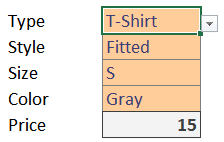
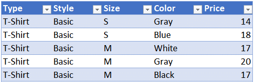
These configuration options all come from a unmarried table, which stores all valid combinations. Perhaps something similar this (Table1):

To create this, we'll use a few functions (SORT, UNIQUE, FILTER) along with information validation.

Video

Narrative

We'll build this using these steps:

Create a drop down list
Repeat for each drop downwards
Recollect related info

Let'due south get to it.

Create a drop down list

Nosotros'll perform 3 steps for each drib down:

Create the listing of choices
Create the in-jail cell driblet downwardly
Make a selection

We'll ultimately repeat these steps for each subsequent drop down.

Create the list of choices

To create the listing of choices, we'll write a formula in an unused surface area of the worksheet.

Let'due south start with the first driblet down, which in our case is Type.

The beginning drop down has no dependencies, and thus will include the same list of choices all the time. Since the products table is named Table1, and the first drop down needs to provide a unique list of all items establish in the Type column, we'll use the following formula:

=UNIQUE(Table1[Type])

Nosotros write the formula into cell B17 and hit Enter. We run across that the formula returns multiple results:

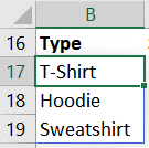
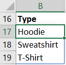
If we'd similar the list to be sorted, we tin include the SORT function in our formula like this:

=SORT(UNIQUE(Table1[Type]))

Now our listing of choices is sorted, like this:

With our listing of choices set, we only demand to get them into an in-jail cell driblet downwardly. For this, we'll apply Data Validation.

Create the in-prison cell drib down

We select the input jail cell, and utilize Data > Data Validation. We allow a list, and prepare the source to =$B$17# similar this:

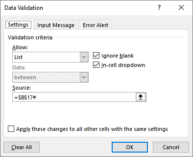
Notation: the # tells Excel to include all results returned by the formula.

The input prison cell at present contains a drop downwardly with the list of choices.

Make a selection

Although we technically do not need to make a selection from the drop downward right now, it will make the side by side pace easier if we exercise. So, we select the input cell and pick any choice so that the cell is not empty, like this:

Note: the reason we make a selection is to avoid formula errors that could lead u.s.a. to believe our formula is wrong.

Echo for each drop down

Then, we perform these steps once again for each subsequent driblet down. We demand to write a formula to create the list of choices, utilize data validation to create the drop down, and then make a selection and so the cell is non empty.

But, at that place is a catch. Each subsequent list of choices depends on the option fabricated in the previous input cell. To accommodate this dependency, we'll use the FILTER role.

Style Drop Down

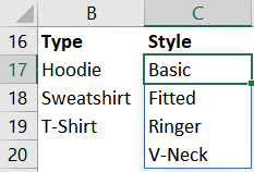
The next choice list is for Fashion. The choices for Mode depend on the selection in the Type input cell. So, to create our listing of Manner choices, we use this formula:

=SORT(UNIQUE(FILTER(Table1[Manner],Table1[Type]=C6)))

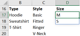
This basically tells Excel to render a sorted listing of unique Style values where the Type cavalcade is equal to the selected Type in C6. We write the formula in C17 and hit Enter:

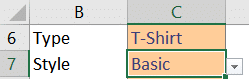
To become that listing of choices into the Way input cell, nosotros once again utilize Data Validation. This time, the source is =$C$17#. We expand the resulting Fashion drib downwards and make a selection so the cell is not blank:

The adjacent input cell is for Size.

Size Drib Down

For Size, our list of choices depends on the values selected for Type and Style.

So, our FILTER role will evidence the list of Sizes where Type and Way values match. To use AND logic when we accept multiple conditions, nosotros employ a multiplication operator * like this:

=SORT(UNIQUE(   FILTER(Table1[Size],(Table1[Way]=C7)*(Table1[Type]=C6)) ))

Note: to use OR logic instead of AND logic, we would use the addition operator + instead of the multiplication operator.

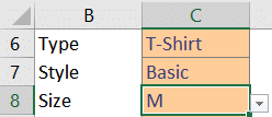
We write the formula into jail cell D17 and hit Enter:

To create the drop down, nosotros employ Information Validation and prepare the source =$D$17#. We expand the resulting drop down and make a option, like this:

And then far so good … we but have 1 final drop down.

Color Drop Downwards

The final drop down for this analogy is color, but you can continue using this same technique for as many drop downs equally needed.

Our formula to create the choices includes conditions for Type, Style and Size:

=SORT(UNIQUE(   FILTER(Table1[Colour],     (Table1[Size]=C8)*(Table1[Fashion]=C7)*(Table1[Type]=C6)     ) ))

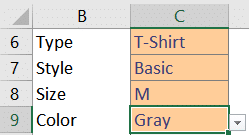
Nosotros write the formula into E17 and hit Enter:

We utilise Information Validation to create the drop downwardly, and set the source =$East$17#. We make a choice:

Now that we have created the dependent drop downs, we tin optionally return related values.

Retrieve related info

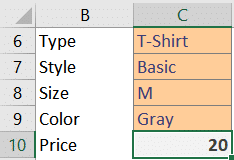
In our case, one time the user has selected the Type, Manner, Size, and Color, we'd like Excel to return the related Cost.

Once once again, we'll turn to the FILTER function. We write the following formula into C10:

=FILTER(Table1[Price],   (Table1[Color]=C9)*(Table1[Size]=C8)*(Table1[Style]=C7)*(Table1[Type]=C6) )

We hit Enter, and bam:

Note: if the products table contained multiple matching rows, we tin can aggregate the results with a helper function such as SUM, MIN, MAX, TEXTJOIN, Average, COUNT, and then on.

If you run into whatever #CALC! errors, information technology probably ways that the dependent input cells are blank, or that the options selected don't have related values. This could happen if you alter the selection in the first input jail cell and don't selection valid options from the updated drib downs for the subsequent cells.

Determination

I think nosotros accomplished our goal. Nosotros created a serial of dependent drop downs. Nosotros used a few functions (FILTER, UNIQUE, SORT) and data validation. Let me know what you call up by posting a comment below … thanks!

Sample file